Credit Modeling with Dask complex task graphs in the real world

This post explores a real-world use case calculating complex credit models in Python using Dask. It is an example of a complex parallel system that is well outside of the traditional “big data” workloads.

This is a guest post

Hi All,

This is a guest post from Rich Postelnik, an Anaconda employee who works with a large retail bank on their credit modeling system. They’re doing interesting work with Dask to manage complex computations (see task graph below). This is a nice example of using Dask for complex problems that are neither a big dataframe nor a big array, but are still highly parallel. Rich was kind enough to write up this description of their problem and share it here.

Thanks Rich!

This is cross-posted at Anaconda’s Developer Blog.

P.S. If others have similar solutions and would like to share them I’d love to host those on this blog as well.

The Problem

When applying for a loan, like a credit card, mortgage, auto loan, etc., we want to estimate the likelihood of default and the profit (or loss) to be gained. Those models are composed of a complex set of equations that depend on each other. There can be hundreds of equations each of which could have up to 20 inputs and yield 20 outputs. That is a lot of information to keep track of! We want to avoid manually keeping track of the dependencies, as well as messy code like the following Python function:

def final_equation(inputs):
    out1 = equation1(inputs)
    out2_1, out2_2, out2_3 = equation2(inputs, out1)
    out3_1, out3_2 = equation3(out2_3, out1)
    ...
    out_final = equation_n(inputs, out,...)
    return out_final

This boils down to a dependency and ordering problem known as task scheduling.

DAGs to the rescue

A directed acyclic graph (DAG) is commonly used to solve task scheduling problems. Dask is a library for delayed task computation that makes use of directed graphs at its core. dask.delayed is a simple decorator that turns a Python function into a graph vertex. If I pass the output from one delayed function as a parameter to another delayed function, Dask creates a directed edge between them. Let’s look at an example:

def add(x, y):
    return x + y

>>> add(2, 2)
4

So here we have a function to add two numbers together. Let’s see what happens when we wrap it with dask.delayed:

>>> add = dask.delayed(add)
>>> left = add(1, 1)
>>> left
Delayed('add-f6204fac-b067-40aa-9d6a-639fc719c3ce')

add now returns a Delayed object. We can pass this as an argument back into our dask.delayed function to start building out a chain of computation.

>>> right = add(1, 1)
>>> four = add(left, right)
>>> four.compute()
4

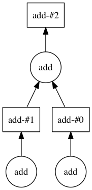
>>> four.visualize()

Below we can see how the DAG starts to come together.

Mock credit example

Let’s assume I’m a mortgage bank and have 10 people applying for a mortgage. I want to estimate the group’s average likelihood to default based on years of credit history and income.

hist_yrs = range(10)
incomes = range(10)

Let’s also assume that default is a function of the incremented years history and half the years experience. While this could be written like:

def default(hist, income):
    return (hist + 1) ** 2 + (income / 2)

I know in the future that I will need the incremented history for another calculation and want to be able to reuse the code as well as avoid doing the computation twice. Instead, I can break those functions out:

from dask import delayed

@delayed
def increment(x):
    return x + 1

@delayed
def halve(y):
    return y / 2

@delayed
def default(hist, income):
    return hist**2 + income

Note how I wrapped the functions with delayed. Now instead of returning a number these functions will return a Delayed object. Even better is that these functions can also take Delayed objects as inputs. It is this passing of Delayed objects as inputs to other delayed functions that allows Dask to construct the task graph. I can now call these functions on my data in the style of normal Python code:

inc_hist = [increment(n) for n in hist_yrs]
halved_income = [halve(n) for n in income]
estimated_default = [default(hist, income) for hist, income in zip(inc_hist, halved_income)]

If you look at these variables, you will see that nothing has actually been calculated yet. They are all lists of Delayed objects.

Now, to get the average, I could just take the sum of estimated_default but I want this to scale (and make a more interesting graph) so let’s do a merge-style reduction.

@delayed
def agg(x, y):
    return x + y

def merge(seq):
    if len(seq) < 2:
        return seq
    middle = len(seq)//2
    left = merge(seq[:middle])
    right = merge(seq[middle:])
    if not right:
        return left
    return [agg(left[0], right[0])]

default_sum = merge(estimated_defaults)

At this point default_sum is a list of length 1 and that first element is the sum of estimated default for all applicants. To get the average, we divide by the number of applicants and call compute:

avg_default = default_sum[0] / 10
avg_default.compute()  # 40.75

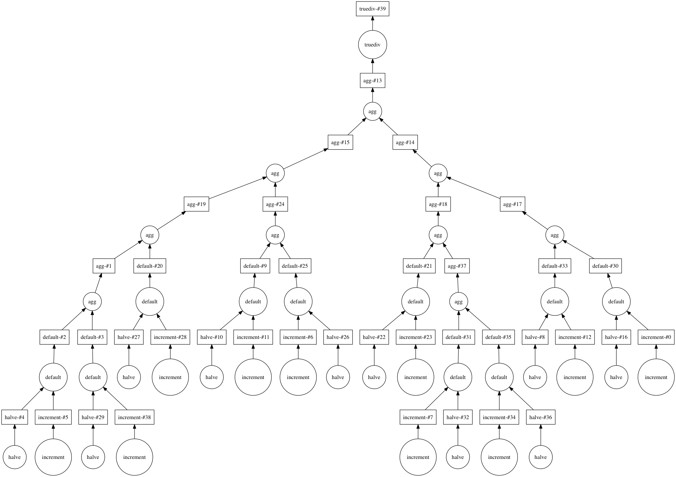
To see the computation graph that Dask will use, we call visualize:

avg_default.visualize()

And that is how Dask can be used to construct a complex system of equations with reusable intermediary calculations.

How we used Dask in practice

For our credit modeling problem, we used Dask to make a custom data structure to represent the individual equations. Using the default example above, this looked something like the following:

class Default(Equation):
    inputs = ['inc_hist', 'halved_income']
    outputs = ['defaults']

    @delayed
    def equation(self, inc_hist, halved_income, **kwargs):
        return inc_hist**2 + halved_income

This allows us to write each equation as its own isolated function and mark its inputs and outputs. With this set of equation objects, we can determine the order of computation (with a topological sort) and let Dask handle the graph generation and computation. This eliminates the onerous task of manually passing around the arguments in the code base. Below is an example task graph for one particular model that the bank actually does.

This graph was a bit too large to render with the normal my_task.visualize() method, so instead we rendered it with Gephi to make the pretty colored graph above. The chaotic upper region of this graph is the individual equation calculations. Zooming in we can see the entry point, our input pandas DataFrame, as the large orange circle at the top and how it gets fed into many of the equations.

The output of the model is about 100 times the size of the input so we do some aggregation at the end via tree reduction. This accounts for the more structured bottom half of the graph. The large green node at the bottom is our final output.

Final Thoughts

With our Dask-based data structure, we spend more of our time writing model code rather than maintenance of the engine itself. This allows a clean separation between our analysts that design and write our models, and our computational system that runs them. Dask also offers a number of advantages not covered above. For example, with Dask you also get access to diagnostics such as time spent running each task and resources used. Also, you can easily distribute your computation with dask distributed with relative ease. Now if I want to run our model across larger-than-memory data or on a distributed cluster, we don’t have to worry about rewriting our code to incorporate something like Spark. Finally, Dask allows you to give pandas-capable business analysts or less technical folks access to large datasets with the dask dataframe.

Full Example

from dask import delayed


@delayed
def increment(x):
    return x + 1


@delayed
def halve(y):
    return y / 2


@delayed
def default(hist, income):
    return hist**2 + income


@delayed
def agg(x, y):
    return x + y


def merge(seq):
    if len(seq) < 2:
        return seq
    middle = len(seq)//2
    left = merge(seq[:middle])
    right = merge(seq[middle:])
    if not right:
        return left
    return [agg(left[0], right[0])]


hist_yrs = range(10)
incomes = range(10)
inc_hist = [increment(n) for n in hist_yrs]
halved_income = [halve(n) for n in incomes]
estimated_defaults = [default(hist, income) for hist, income in zip(inc_hist, halved_income)]
default_sum = merge(estimated_defaults)
avg_default = default_sum[0] / 10
avg_default.compute()
avg_default.visualize()  # requires graphviz and python-graphviz to be installed

Acknowledgements

Special thanks to Matt Rocklin, Michael Grant, Gus Cavanagh, and Rory Merritt for their feedback when writing this article.