Distributed Dask Arrays

This work is supported by Continuum Analytics and the XDATA Program as part of the Blaze Project

In this post we analyze weather data across a cluster using NumPy in parallel with dask.array. We focus on the following:

How to set up the distributed scheduler with a job scheduler like Sun GridEngine.
How to load NetCDF data from a network file system (NFS) into distributed RAM
How to manipulate data with dask.arrays
How to interact with distributed data using IPython widgets

This blogpost has an accompanying screencast which might be a bit more fun than this text version.

This is the third in a sequence of blogposts about dask.distributed:

Setup

We wanted to emulate the typical academic cluster setup using a job scheduler like SunGridEngine (similar to SLURM, Torque, PBS scripts and other technologies), a shared network file system, and typical binary stored arrays in NetCDF files (similar to HDF5).

To this end we used Starcluster, a quick way to set up such a cluster on EC2 with SGE and NFS, and we downloaded data from the European Centre for Meteorology and Weather Forecasting

To deploy dask’s distributed scheduler with SGE we made a scheduler on the master node:

sgeadmin@master:~$ dscheduler
distributed.scheduler - INFO - Start Scheduler at:  172.31.7.88:8786

And then used the qsub command to start four dask workers, pointing to the scheduler address:

sgeadmin@master:~$ qsub -b y -V dworker 172.31.7.88:8786
Your job 1 ("dworker") has been submitted
sgeadmin@master:~$ qsub -b y -V dworker 172.31.7.88:8786
Your job 2 ("dworker") has been submitted
sgeadmin@master:~$ qsub -b y -V dworker 172.31.7.88:8786
Your job 3 ("dworker") has been submitted
sgeadmin@master:~$ qsub -b y -V dworker 172.31.7.88:8786
Your job 4 ("dworker") has been submitted

After a few seconds these workers start on various nodes in the cluster and connect to the scheduler.

Load sample data on a single machine

On the shared NFS drive we’ve downloaded several NetCDF3 files, each holding the global temperature every six hours for a single day:

>>> from glob import glob
>>> filenames = sorted(glob('*.nc3'))
>>> filenames[:5]
['2014-01-01.nc3',
 '2014-01-02.nc3',
 '2014-01-03.nc3',
 '2014-01-04.nc3',
 '2014-01-05.nc3']

We use conda to install the netCDF4 library and make a small function to read the t2m variable for “temperature at two meters elevation” from a single filename:

conda install netcdf4

import netCDF4
def load_temperature(fn):
    with netCDF4.Dataset(fn) as f:
        return f.variables['t2m'][:]

This converts a single file into a single numpy array in memory. We could call this on an individual file locally as follows:

>>> load_temperature(filenames[0])
array([[[ 253.96238624,  253.96238624,  253.96238624, ...,  253.96238624,
          253.96238624,  253.96238624],
        [ 252.80590921,  252.81070124,  252.81389593, ...,  252.79792249,
          252.80111718,  252.80271452],
          ...
>>> load_temperature(filenames[0]).shape
(4, 721, 1440)

Our dataset has dimensions of (time, latitude, longitude). Note above that each day has four time entries (measurements every six hours).

The NFS set up by Starcluster is unfortunately quite small. We were only able to fit around five months of data (136 days) in shared disk.

Load data across cluster

We want to call the load_temperature function on our list filenames on each of our four workers. We connect a dask Executor to our scheduler address and then map our function on our filenames:

>>> from distributed import Executor, progress
>>> e = Executor('172.31.7.88:8786')
>>> e
<Executor: scheduler=172.31.7.88:8786 workers=4 threads=32>

>>> futures = e.map(load_temperature, filenames)
>>> progress(futures)

After this completes we have several numpy arrays scattered about the memory of each of our four workers.

Coordinate with dask.array

We coordinate these many numpy arrays into a single logical dask array as follows:

>>> from distributed.collections import futures_to_dask_arrays
>>> xs = futures_to_dask_arrays(futures)  # many small dask arrays

>>> import dask.array as da
>>> x = da.concatenate(xs, axis=0)        # one large dask array, joined by time
>>> x
dask.array<concate..., shape=(544, 721, 1440), dtype=float64, chunksize=(4, 721, 1440)>

This single logical dask array is comprised of 136 numpy arrays spread across our cluster. Operations on the single dask array will trigger many operations on each of our numpy arrays.

Interact with Distributed Data

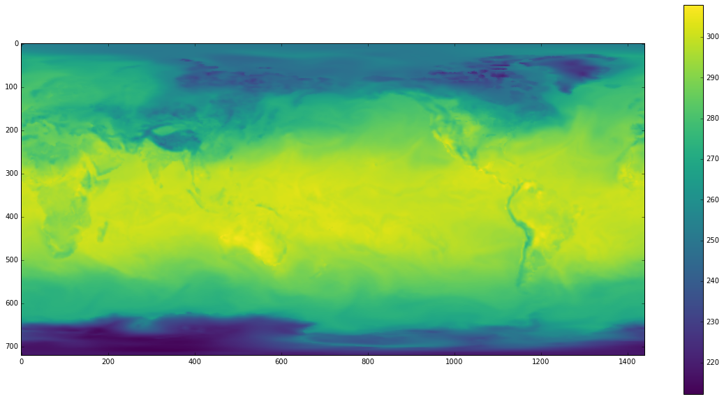
We can now interact with our dataset using standard NumPy syntax and other PyData libraries. Below we pull out a single time slice and render it to the screen with matplotlib.

from matplotlib import pyplot as plt
plt.imshow(x[100, :, :].compute(), cmap='viridis')
plt.colorbar()

In the screencast version of this post we hook this up to an IPython slider widget and scroll around time, which is fun.

Speed

We benchmark a few representative operations to look at the strengths and weaknesses of the distributed system.

Single element

This single element computation accesses a single number from a single NumPy array of our dataset. It is bound by a network roundtrip from client to scheduler, to worker, and back.

>>> %time x[0, 0, 0].compute()
CPU times: user 4 ms, sys: 0 ns, total: 4 ms
Wall time: 9.72 ms

Single time slice

This time slice computation pulls around 8 MB from a single NumPy array on a single worker. It is likely bound by network bandwidth.

>>> %time x[0].compute()
CPU times: user 24 ms, sys: 24 ms, total: 48 ms
Wall time: 274 ms

Mean computation

This mean computation touches every number in every NumPy array across all of our workers. Computing means is quite fast, so this is likely bound by scheduler overhead.

>>> %time x.mean().compute()
CPU times: user 88 ms, sys: 0 ns, total: 88 ms
Wall time: 422 ms

Interactive Widgets

To make these times feel more visceral we hook up these computations to IPython Widgets.

This first example looks fairly fluid. This only touches a single worker and returns a small result. It is cheap because it indexes in a way that is well aligned with how our NumPy arrays are split up by time.

@interact(time=[0, x.shape[0] - 1])
def f(time):
    return x[time, :, :].mean().compute()

This second example is less fluid because we index across our NumPy chunks. Each computation touches all of our data. It’s still not bad though and quite acceptable by today’s standards of interactive distributed data science.

@interact(lat=[0, x.shape[1] - 1])
def f(lat):
    return x[:, lat, :].mean().compute()

Normalize Data

Until now we’ve only performed simple calculations on our data, usually grabbing out means. The image of the temperature above looks unsurprising. The image is dominated by the facts that land is warmer than oceans and that the equator is warmer than the poles. No surprises there.

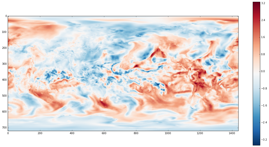
To make things more interesting we subtract off the mean and divide by the standard deviation over time. This will tell us how unexpectedly hot or cold a particular point was, relative to all measurements of that point over time. This gives us something like a geo-located Z-Score.

z = (x - x.mean(axis=0)) / x.std(axis=0)
z = e.persist(z)
progress(z)

plt.imshow(z[slice].compute(), cmap='RdBu_r')
plt.colorbar()

We can now see much more fine structure of the currents of the day. In the screencast version we hook this dataset up to a slider as well and inspect various times.

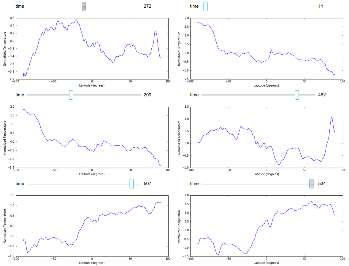
I’ve avoided displaying GIFs of full images changing in this post to keep the size down, however we can easily render a plot of average temperature by latitude changing over time here:

import numpy as np
xrange = 90 - np.arange(z.shape[1]) / 4

@interact(time=[0, z.shape[0] - 1])
def f(time):
    plt.figure(figsize=(10, 4))
    plt.plot(xrange, z[time].mean(axis=1).compute())
    plt.ylabel("Normalized Temperature")
    plt.xlabel("Latitude (degrees)")

Conclusion

We showed how to use distributed dask.arrays on a typical academic cluster. I’ve had several conversations with different groups about this topic; it seems to be a common case. I hope that the instructions at the beginning of this post prove to be helpful to others.

It is really satisfying to me to couple interactive widgets with data on a cluster in an intuitive way. This sort of fluid interaction on larger datasets is a core problem in modern data science.

What didn’t work

As always I’ll include a section like this on what didn’t work well or what I would have done with more time:

No high-level read_netcdf function: We had to use the mid-level API of executor.map to construct our dask array. This is a bit of a pain for novice users. We should probably adapt existing high-level functions in dask.array to robustly handle the distributed data case.
Need a larger problem: Our dataset could have fit into a Macbook Pro. A larger dataset that could not have been efficiently investigated from a single machine would have really cemented the need for this technology.
Easier deployment: The solution above with qsub was straightforward but not always accessible to novice users. Additionally while SGE is common there are several other systems that are just as common. We need to think of nice ways to automate this for the user.
XArray integration: Many people use dask.array on single machines through XArray, an excellent library for the analysis of labeled nd-arrays especially common in climate science. It would be good to integrate this new distributed work into the XArray project. I suspect that doing this mostly involves handling the data ingest problem described above.
Reduction speed: The computation of normalized temperature, z, took a surprisingly long time. I’d like to look into what is holding up that computation.